knitr::opts_chunk$set(echo = TRUE)
#Vectors
age = c(22,21,24,19,20,23)
age
age[2]
yrs_math_ed = c(4,5,2,5,3,5)
yrs_math_ed
#data frames
df1 = data.frame(Age = age, Years = yrs_math_ed)
df1
df1[4,2] #Data in the 4th row and 2nd column
df1[1,] #all the data in the 1st row
df1$Math_Level #all the data in the fourth column
a = c("Mary","Martha","Kim","Kristen","Amy","Sam")
b = c("English","Math","Sociology","Math","Music","Dance")
#Make a data frame
df2 = data.frame(Name = a, Major = b)
df2
#Make another data frame
df3 = data.frame(Age = age, Years = yrs_math_ed,Name = a, Major = b)
df3
#Cbind combines columns
df4 = cbind(df1,df2)
df4
#str and class show what type of variable it is
str(df4)
class(df4$Name)
summary(df4)
#define a new row / student
d = c(19,4,"John","Math")
#attempt to add a row
df5 = rbind(df4,d) #problem here is that Name and Major are factors
#try and fix the problem
dfCopy = df4
dfCopy$Name = as.character(df4$Name)
dfCopy$Major = as.character(df4$Major)
summary(dfCopy)
#add the student to the end of the data frame.
df5 = rbind(dfCopy,d)
df5
#recheck the class
str(df5)
summary(df5)
#fix the classes
df5$Age = as.numeric(df5$Age)
df5$Years = as.numeric(df5$Years)
summary(df5)
df5$Name = as.factor(df5$Name)
df5$Major = as.factor(df5$Major)
summary(df5)
#Filter the data frame
#All students with more than 4 years of Math
df5[df5$Years > 4,]
#All students with more than 4 years of Math and are 21 years of age or older
df5[(df5$Age >= 21 & df5$Years > 4), ]
#All students that are majoring in Math
df5[df5$Major == "Math",]
Example1 = read.csv("../btobin0.github.io.git/BusinessSales.csv",header = TRUE)
Example1$sales
# iris is Edgar Anderson's Iris Data
str(iris) # get type and other variable information
head(iris) #look at first 6 rows
tail(iris) #look at last 6 rows.
iris$Sepal.Width # look at all Sepal.Widths
#install.packages("ggplot2") # I have already installed this package... you only need install the package once.
library(ggplot2) #However, you need to laod the library each time you start a new session.
?mpg #mpg info and note that it is a tibble.
str(mpg) # get type and other variable information
head(mpg) #look at first 6 rows.
mpg$cty #look at all city mpg values.
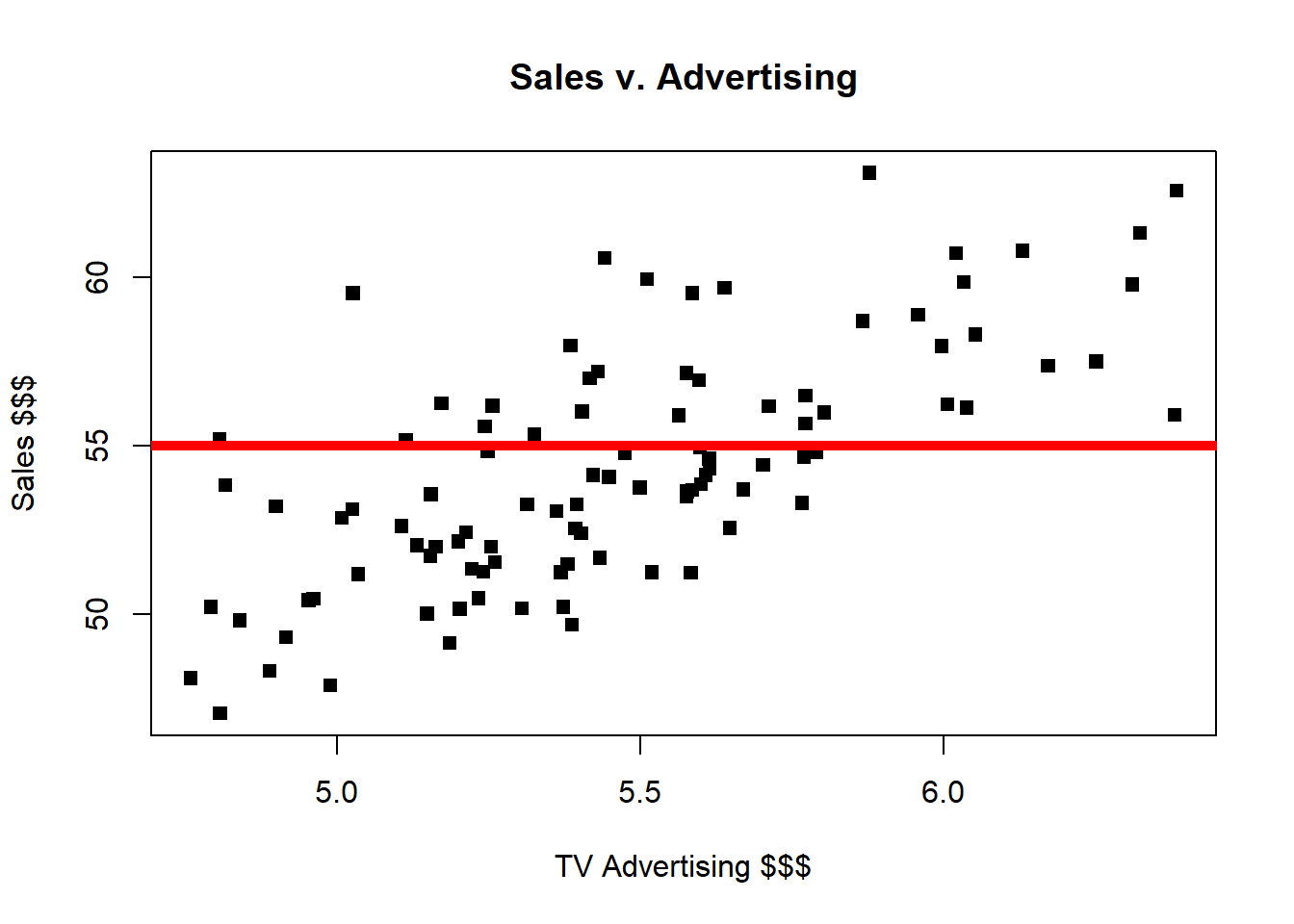
Example1 = read.csv("../btobin0.github.io.git/BusinessSales.csv",header = TRUE)
head(Example1)
#plot(x,y,col,pch,type,ylab,xlab,main)
plot(Example1$ad_tv,Example1$sales, pch = 15,xlab = "TV Advertising $$$",ylab = "Sales $$$", main = "Sales v. Advertising")
abline(h = 55, col = "red",lwd = 5)
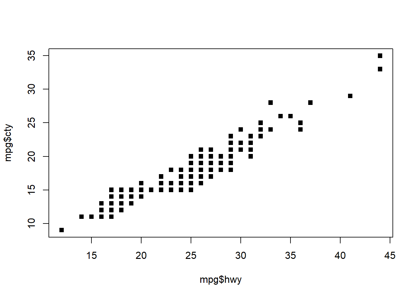
plot(mpg$hwy,mpg$cty,pch = 15) #NO LABLES ... AHHH!!!
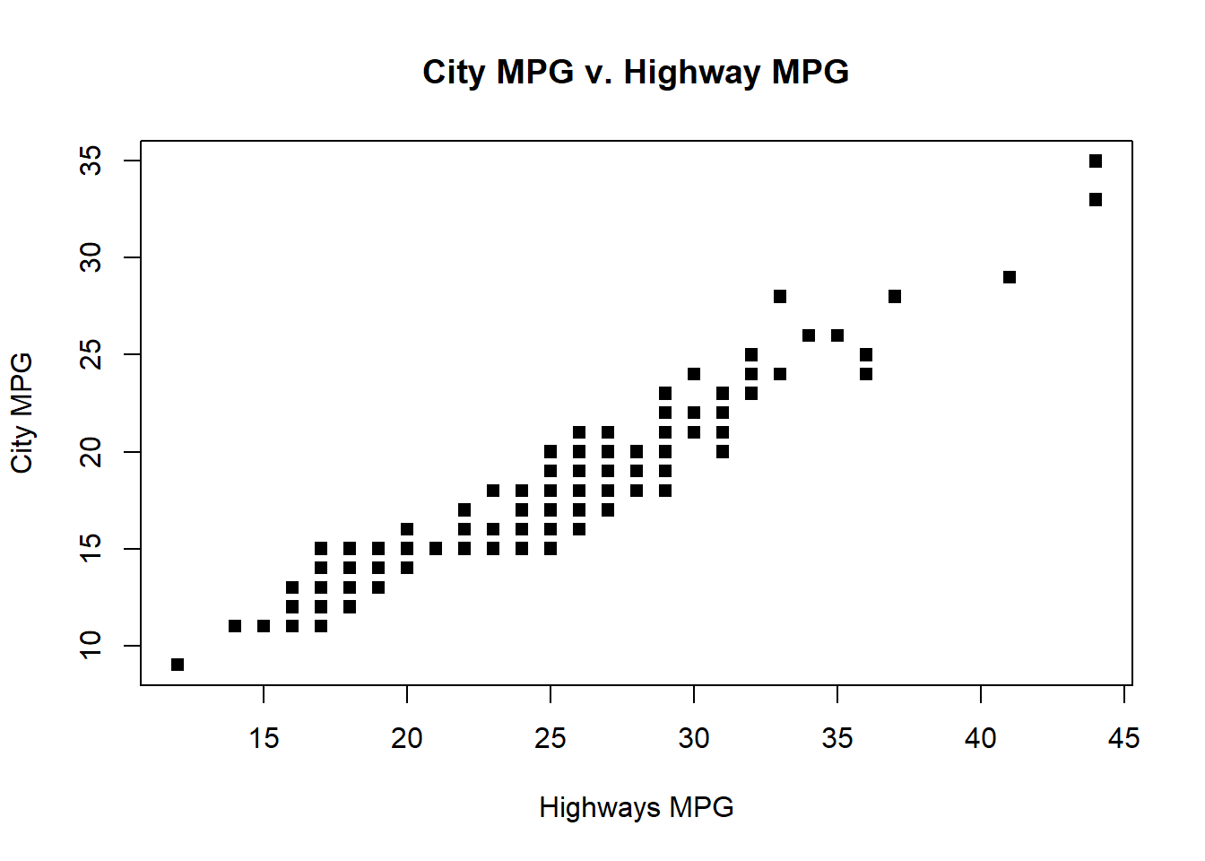
plot(mpg$hwy,mpg$cty,pch = 15, main = "City MPG v. Highway MPG", ylab = "City MPG", xlab = "Highways MPG")
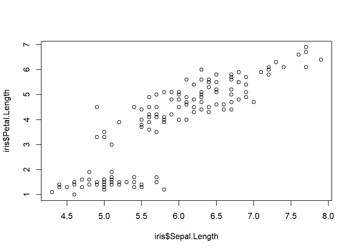
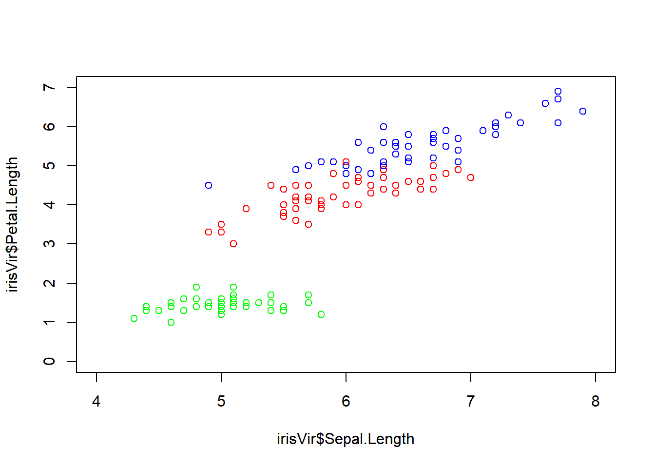
plot(iris$Sepal.Length,iris$Petal.Length) #note domain and range of plot
irisVir = iris[iris$Species == "virginica",]
plot(irisVir$Sepal.Length,irisVir$Petal.Length, col = "blue", ylim = c(0,7), xlim = c(4,8))
irisVers = iris[iris$Species == "versicolor",]
points(irisVers$Sepal.Length,irisVers$Petal.Length, col = "Red")
irisSet = iris[iris$Species == "setosa",]
points(irisSet$Sepal.Length,irisSet$Petal.Length, col = "green")
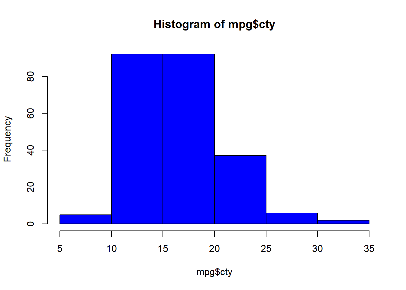
hist(mpg$cty,col = "blue")
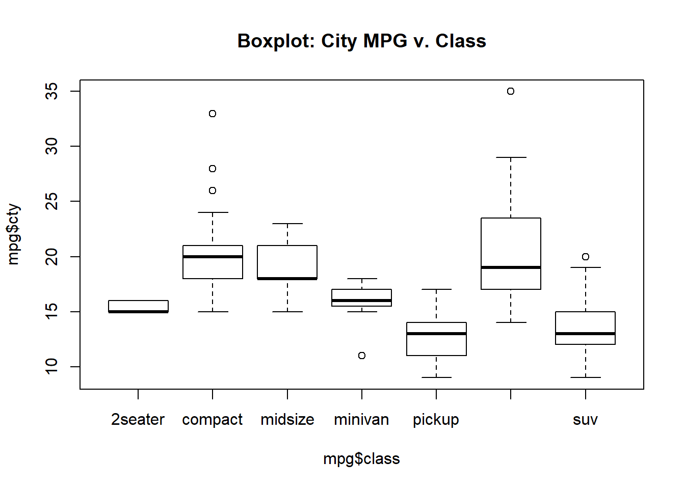
boxplot(mpg$cty~mpg$class, main = "Boxplot: City MPG v. Class")
dev.off()

par(mfrow = c(1,2))

hist(mpg$cty,col = "blue", main = "Histogram of MPG", xlab = "MPG")
boxplot(mpg$cty~mpg$class, data= mpg, main = "Boxplot of MPG by Class", xlab = "Cylinder")


### You Try it! Make a histogram of the Iris Sepal Lengths
### Comment on the distribution (skewness?  number of modes? etc.)


hist(iris$Petal.Length, col = "blue", main = "Histogram of Iris Sepal Lengths")

age = c(22,21,24,19,20,23)
yrs_math_ed = c(4,5,2,5,3,5)
names = c("Mary","Martha","Kim","Kristen","Amy","Sam")
subject = c("English","Math","Sociology","Math","Music","Dance")

df3 = data.frame(Age = age, Years = yrs_math_ed, Name = names, Subject = subject)

barplot(df3$Years, names.arg = df3$Name)

summary(mpg$class)

mpg$classFact = as.factor(mpg$class)
head(mpg)
summary(mpg$classFact)

barplot(summary(mpg$classFact))

#draw a sample from a standard normal distribution
#run many times varying sample size and look at histogram and mean
sample1 = rnorm(1000,0,1)
hist(sample1)
mean(sample1)
sd(sample1)

population = rnorm(10000000,0,1) #note the the number of draws here
hist(population)
sample1 = sample(population,100) #sample of size 100
hist(sample1)
mean(sample1)
sd(sample1)

xBarVec = c() #Global vector to hold the sample means
population = rnorm(10000000,0,1) #Simulating the population

#####################################################
# Funciton: xbarGenerator
# Argements: samplesize: the size of the sample that each sample mean is based on.
#            number_of_samples: the number of samples and thus sample means we will generate
# Author: Bivin Sadler
#####################################################
xbarGenerator = function(sampleSize = 30,number_of_samples = 100)
{
  for(i in 1:number_of_samples)
  {
    theSample = sample(population,sampleSize)
    xbar = mean(theSample)
    xBarVec = c(xBarVec, xbar)
  }
  return(xBarVec)
}

xbars = xbarGenerator(30,1000)
length(xbars)
hist(xbars)

xBarVec = c() #global vector to hold the sample means
#####################################################
# Funciton: xbarGenerator (Adpated)
# Argements: samplesize: the size of the sample that each sample mean is based on.
#            number_of_samples: the number of samples and thus sample means we will generate
# Author: Bivin Sadler
#####################################################
xbarGenerator2 = function(sampleSize = 30,number_of_samples = 100, mean = 0, sd = 1)
{
  for(i in 1:number_of_samples)
  {
    theSample = rnorm(sampleSize,mean,sd)
    xbar = mean(theSample)
    xBarVec = c(xBarVec, xbar)
  }
  return(xBarVec)
}

xbars = xbarGenerator2(60,1000,50,10)
hist(xbars)
summary(xbars)
sd(xbars)
10/sqrt(60)